on
Data analysis around Jelly Party
The Status Quo
Jelly Party currently features ~5000 active users. While growth has been small during August, Winter is coming and with it, growth returns. At this stage Jelly Party is still growing entirely organic, as there is zero marketing around Jelly Party.
Obtaining data
The Jelly Party Server constantly pushes anonymized data into an elasticsearch server using filebeat. This information includes Geo-IP data, avatar information, the number of active parties & clients and the redirect URL. The redirect URL is of particular interest, because it tells us what hosts people use Jelly-Party on. Furthermore, we can compute session-metrics, using join- and leave-timestamps.
Connecting to elasticsearch
It turns out that we can query data from elasticsearch using a native Python library.
from elasticsearch import Elasticsearch
from elasticsearch.helpers import scan
import json
import os

if not os.environ['ELASTIC_PASSWORD'] or not os.environ['ELASTIC_HOST']:
    raise RuntimeError("MUST PROVIDE ELASTIC HOST & PASSWORD")

es = Elasticsearch(
    os.environ['ELASTIC_HOST'],
    http_auth=('elastic', os.environ['ELASTIC_PASSWORD']),
    scheme="https",
    port=9200,
)

es.info()
Downloading data
Once connected, we can recursively query data from elasticsearch, saving each data entry into a list called items. Luckily we’re still in a position to greedily load all data into RAM.
es_response = scan(
    es,
    index='filebeat*',
    query={"query": { "match_all" : {}}}
)

items = []
for item in es_response:
    items.append(item)
Parsing data into pandas
Next, we use pandas to parse our data in to a easily processable dataframe. We must first flatten our items array, which is a nested JSON object. Also, we set the _source.@timestamp as a datetime-index, drop columns that we’re not interested in and throw out any rows that contain only NaN-s.
import pandas as pd

mdf = pd.json_normalize(items)
index = pd.to_datetime(mdf["_source.@timestamp"])
mdf = mdf.set_index(index)
raw_mdf = mdf.copy()
# Drop all columns but a few select ones
drop_cols = []
for col in mdf.columns:
    if not any(e in col for e in ["_source.message_decoded", "activeClients", "activeParties"]):
        drop_cols.append(col)
mdf = mdf.drop(drop_cols, axis=1, errors="ignore")
mdf = mdf.dropna(axis=0, how="all")
mdf = mdf.sort_index()
Let’s use pickle to dump our objects to local storage, to save us from having to download data again.
import pickle

with open("./raw.pickle", "wb") as f:
    pickle.dump(raw_mdf, f)
with open("./df.pickle", "wb") as f:
    pickle.dump(mdf, f)
Creating a dataframe that contains only join-entries is as simple as indexing into our original dataframe.
join = mdf[mdf["_source.message_decoded.type"] == "join"]
Reverting URI encodings
Our redirectURL is a messy string, e.g. https://join.jelly-party.com/?redirectURL=https%253A%252F%252Fwww.youtube.com%252Fwatch%253Fv%253DoOYA-jsWTmc&jellyPartyId=smart-contraries-border-firmly.
This string has undergone several URI-encodings, which we must revert to extract the host. We build a simple function to extract the netloc, path & query.
import urllib
import numpy as np

def passURL(d, get):
    try:
        data = urllib.parse.urlparse(urllib.parse.unquote(urllib.parse.parse_qs(urllib.parse.urlparse(d)[4])["redirectURL"][0]))
        if get == "netloc":
            return data.netloc
        elif get == "path":
            return data.path
        else:
            return data.query
    except:
        return np.nan
We can now use this function and pandas transform-method to create a dataframe that extracts netloc, path and query.
urls = join["_source.message_decoded.data.clientState.currentlyWatching"]
urls = urls.transform([lambda x: passURL(x, "netloc"), lambda x: passURL(x, "path"), lambda x: passURL(x, "query")])
urls.columns = ["netloc", "path", "query"]
Generating Insights
Now that we have the data at hand, let’s start with some simple analysis.
Most used websites
Using pandas built-in value_counts-method, we can identify most-used websites.
urls["netloc"].value_counts().iloc[:12]
This returns the top 12 websites Jelly Party has been used on, indicating the no. of sessions to the right:
www.primevideo.com         33266
www.netflix.com             27758
www.youtube.com            26484
www.hotstar.com             7151
www.disneyplus.com          5904
play.stan.com.au            5305
www.amazon.com              5030
www.amazon.co.uk            4376
www.hulu.com                2935
www.viki.com                2786
soap2day.to                 1830
www.crave.ca                1464
Computing site metrics
Unsurprisingly, people use Jelly Party on all kinds of websites. However, there have been numerous reports that certain websites don’t function, and many of these sites can be found in the data. Let’s compute some website metrics to shed light on this.
We start by filtering our dataframe for join and disconnect message types. We then throw away all columns, but the session unique uuids and the currentlyWatching string (which we must, once again, dissect the netloc from — it comes helpful that we previously built a helper function for this).
Lastly, we group by uuids and then aggregate data using a custom aggregator function. We also use our previously defined passURL function to extract the netloc from the redirectURL.
join_leave = mdf[(mdf["_source.message_decoded.type"] == "join") | (mdf["_source.message_decoded.type"] == "disconnect")][["_source.message_decoded.data.clientState.currentlyWatching", "_source.message_decoded.data.uuid"]]
aggregator = {"_source.message_decoded.data.uuid": lambda df: (df.index[-1] - df.index[0]), "_source.message_decoded.data.clientState.currentlyWatching": lambda df: df.iloc[0]}
session_df = join_leave.groupby("_source.message_decoded.data.uuid").agg(aggregator)
session_df['netloc'] = session_df["_source.message_decoded.data.clientState.currentlyWatching"].apply(lambda x: passURL(x, "netloc"))
session_df = session_df.drop(["_source.message_decoded.data.clientState.currentlyWatching"], axis=1)
session_df.columns = ["Session duration", "netloc"]
Sweet. We now have a dataframe containing sessions with duration and netloc. We can use this dataframe to compute some metrics for different hosts. We do this by:
- Grouping by
netloc - Computing group specific metrics
- Pushing the data into a new dataframe
group_obj = session_df.groupby("netloc")
mean = group_obj.apply(lambda df: df["Session duration"].mean().seconds//60).sort_values(ascending=False)
std = group_obj.apply(lambda df: df["Session duration"].std().seconds//60).sort_values(ascending=False)
count = group_obj.apply(lambda df: df["Session duration"].count()).sort_values(ascending=False)
session_metrics = pd.DataFrame(data={"Session duration mean [minutes]": mean, "Session duration Std [minutes]": std, "Count":  count})
session_metrics.loc[urls["netloc"].value_counts().iloc[:12].index.values]
This gets us the following session duration information:
Host                Mean [minutes]      Std [minutes]       Count
www.primevideo.com  31	                55.0	            10539
www.netflix.com	    47	                73.0	            9436
www.youtube.com	    30	                72.0	            9377
www.hotstar.com	    33	                47.0	            2399
www.disneyplus.com	40	                73.0	            1705
play.stan.com.au	54	                58.0	            1900
www.amazon.com	    33	                109.0	            1406
www.amazon.co.uk	45	                73.0	            1235
www.hulu.com	    47	                88.0	            870
www.viki.com	    82	                101.0	            922
soap2day.to	        22	                35.0	            685
www.crave.ca	    69	                77.0	            418
Really, we should vectorize this..
Calling .apply is bad practice, because it doesn’t vectorize computations. Thus, a Todo for later remains to fully vectorize the code. E.g. for computing the mean, this could look as follows:
group_obj = session_df.groupby("netloc", dropna=True)["Session duration"]
group_obj.mean(numeric_only=False)
Plotting histograms
Alright. This is kinda neat, though we aggregate unknown distributions. Let’s plot histograms to visualize the respective distributions a little better. We built a little helper function that accepts a hostname and returns a figure with two histograms, one looking at the [0,120] range and the other one looking at the [10,300] range (we’ll explain why we chose those ranges in a second).
def buildHistogram(host):
    values = session_df.groupby("netloc").get_group(host)["Session duration"].apply(lambda x: x.seconds//60).values
    fig, ax = plt.subplots(2,1,figsize=(14,7), dpi=300)  # Create a figure and an axes.
    ax[0].set_title(f"Session duration histogram for {host} [0-120 minutes]")
    ax[0].set_xlabel(f"Session duration bins")
    ax[0].set_ylabel(f"Session duration [minutes]")
    ax[0].hist(values, bins=20, range=(0.0, 120))
    ax[1].set_title(f"Session duration histogram for {host} [10-300 minutes]")
    ax[1].set_xlabel(f"Session duration bins")
    ax[1].set_ylabel(f"Session duration [minutes]")
    ax[1].hist(values, bins=20, range=(10, 300))
    plt.tight_layout()

buildHistogram("www.netflix.com")
The figure for Netflix looks as follows:
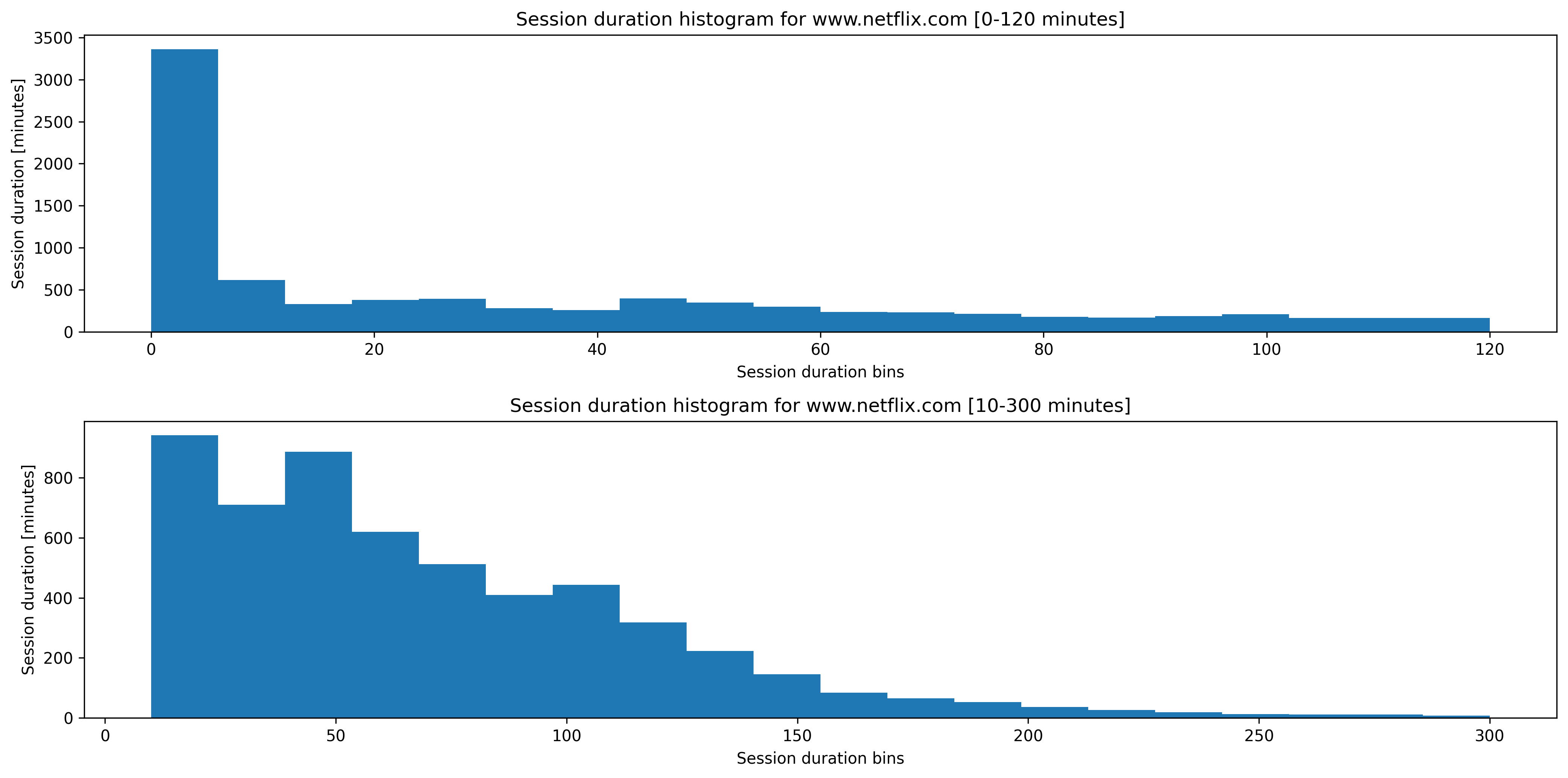
Figure with histograms for Netflix
It turns out that most sessions are very short. This is very odd. Either, there’s a frontend bug that forces users to quit the session and restart it, or we’re being scanned by extension analyzers for possible vulnerabilites. These analyzers must be sophistcated though, as they pick up the Jelly Party protocol. I suppose if you look at the Jelly Party source code, you can inspect Typescript-signatures and thereby extract websocket protocols. Maybe then start fuzzing around this protocol? I know that the server used to crash because connections were made to it using a different protocol than the one it expected. I believe I am still logging this somewhere, so it remains a thing to look into.
Anyways, the magic link joining is indeed kinda buggy and another thing to further look into (unfortunately browser security concepts force a certain pattern that is rather error-prone). However, the personal feedback that I keep collecting does not indicate such a systemic/widespread issue.
The data seems sensible otherwise. E.g. for Youtube, we’d expect shorter session durations, as this aligns with our understanding of how people consume Youtube (watching shorter videos, skipping around, etc.). Also, we generally expect a right-skew of the distribution.
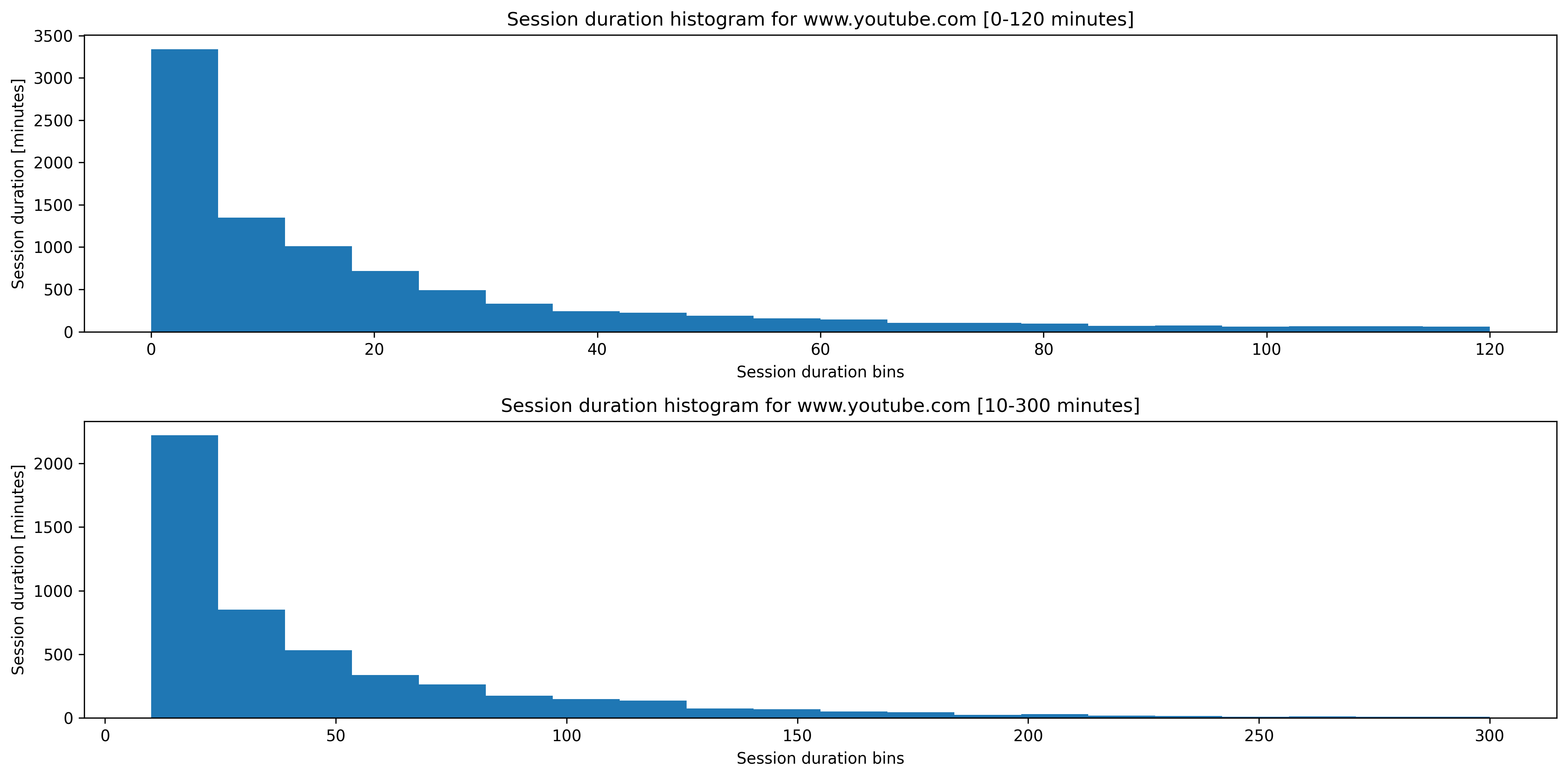
Figure with histograms for Youtube
Identifying broken sites
Let’s see if we can find some broken websites. Our process is the following:
- Filter for websites that have had more than 50 sessions.
- Look at websites with the smallest
mean session duration.
broken_websites_df = session_metrics[session_metrics["Count"] > 50 ]
broken_websites_df.sort_values(by="Session duration mean [minutes]").head(20)
Besides websites that Jelly Party is simply not built for (e.g. https://www.google.com/ or https://www.jelly-party.com/), we find websites such as https://www.crunchyroll.com and https://www3.animeflv.net. Having a quick look at these websites, we notice that they embed videos into yet another iFrame, which explains why the extension doesn’t work on these sites. A solution would be to have a messaging module injected into all frames and then communicate to this module using the background script. We’re currently evaluating if this makes sense, since this is technically rather involved.
Are Youtube sessions shorter than Netflix sessions?
Let’s formulate a simple statistical test to answer this question. Let (µ₁,σ₁) reflect the sample mean and variance of Youtube and (µ₂,σ₂)reflect the sample mean and variance of Netflix, respectively. Our hypothesis thus becomes:
H₀: µ₁ >= µ₂ (Youtube sessions are longer than Netflix sessions)
H₁: µ₁ <  µ₂ (Netflix sessions are longer than Youtube sessions)
We’ll use a t-test (specifically Welch’s t-test) to evaluate our hypothesis. We get the following result:
Ttest_indResult(statistic=17.166169405158687, pvalue=1.5361992613156065e-65)
Since we use Ttest_indResult, which is a two-sided test, but we’re interested in a one-sided test, we must divide our (already neglibibly small) pvalue by 2 (see here why). We still remain correct (at least statistically speaking) in our assumption that Youtube sessions are shorter than Netflix sessions.
Takeaways
There’s a couple of things we learned from our first quick analysis.
- Session durations vary greatly: Most sessions are very short-lived.
- People watch differently on different video platforms. E.g. sessions are shorter on Youtube than on Netflix.
- Some websites are broken. We identified two, which use nested
iFramesfor which we cannot access the video feed.